by Ken Hanawalt, MMR
This document is a supplement to the “On Operations Part 7” column “Making Car Cards” in the June 2025 Div 2 Keystone Flyer, available at https://keystonedivision.org/flyer/Flyer68_06_color_noem.pdf
Use of model railroad car cards is a method to guide the realistic movement of railroad cars during a layout operating session. The method can be implemented using a three part spreadsheet. Sheet 1 holds an inventory file of cars and their intended destinations, Sheet 2 is used to print car-card envelopes to hold waybills, and Sheet 3 is used to print waybills that specify the destinations for cars. You can download the spreadsheet file, LibreOfficeWaybillGenerator V2 Sheets.ods, and execute or modify it to generate car cards for your own layout.
The included spreadsheet is ready to use and is populated with sample data that you can print to see how it works. To use it on your layout, you can replace the Sheet 1 inventory with data about your railroad cars and layout destinations, and then print car cards for your layout without changing the spreadsheet design.
The included spreadsheet is implemented using LibreOffice Calc (available for free download at LibreOffice.com) and is based on ideas proposed by Chris van der Heide, available at: https://vanderheide.ca/blog/2018/01/04/excel-car-cards-and-waybills/. This document describes how the spreadsheet is implemented and how you might modify it if you want different features.
There are several key insights in the article by van der Heide that make this application possible. The main insight is that spreadsheet programs can print text that is rotated to the left or to the right but usually not upside down, so we print the envelopes and waybills sideways on the paper (landscape format). After the waybills are printed and cut apart, we can put them in the envelope right-side up or up-side down to show the destination that we want to use next. The second insight is that the VLOOKUP formula can be used on one page of a spreadsheet to extract and use data from another page. In particular, it is used on the waybill page to read and use data from the inventory page. This means that the same inventory data can be used repeatedly after entering it only once.
When Calc is started, a menu at the bottom of the screen will show the three pages. To select a sheet to work on, click the sheet name. To see or modify the car inventory, use Sheet 1,
Sheet 1 Car Inventory
Sheet 1 of the spreadsheet is used to hold a list of the cars and their layout destinations as shown in the example below. A full description is available in the Flyer column. The essential information is a unique Car ID, a Car Mark to identify each car, and information about the destinations for the cars, normally including a Town Name, Spur Name, and Train Name. The Car ID values are referenced by formulas that select car information to be printed. To change the data to represent your layout, just click on Sheet 1 spreadsheet cells and type in your information. Note: you can use Control-Enter to insert a line break inside a spreadsheet cell as shown in the Car Description and Destination cells. You can use Control-C and Control-V to copy data from one cell to another as in most Windows applications.
Car ID |
Car Mark |
Car Description |
Destination 1 |
Destination 2 |
Destination 3 |
Destination 4 |
1 |
TK AMOX 1260 |
Amoco 40ft Silver Tank ID#1 |
Julius FM Interchange East Branch |
Julius Fuel & Oil East Branch |
Julius FM Interchange East Branch |
Julius Fuel & Oil East Branch |
2 |
BX B&O 455356 |
Baltimore & Ohio 40ft Brown Box ID#2 |
Julius Freight Transfer East Branch |
Julius Ag Supply East Branch |
Julius Machine & Tool East Branch |
Julius Lumber Shed East Branch |
The provided spreadsheet gives a two sided waybill with four available positions. You can use fewer destinations for some cars if you wish, and the unused ones will be blank on the resulting waybills. You will need to modify the spreadsheet to use more than 4 destinations.
Sheet 2 Car-Card Envelope
A major deviation from the van der Heide design is that I prefer to use blank car-card envelopes rather than having car identifications on the envelopes. This approach results from my operations design objective of reducing or eliminating requirements for staging between operating sessions, and it makes the envelopes much easier to design and print, although I actually use cut-down coin envelopes on my layout instead of printing envelopes.
To print blank envelopes without modification, just select Sheet 2 and select File – Print. Most printers will let you specify how many copies to make. Each copy will contain six envelopes. These can be cut apart on the solid lines after printing, and folded on the dotted lines. After folding, the smaller flap can be taped to the sides of the taller part to make the envelope. Waybills printed using Sheet 3 will fit inside the envelope, showing only one destination at a time.
Following are the steps that I used to create this sheet using LibreOffice Calc and some suggestions on how to modify it if desired.
Set up the basic page format
Open LibreOffice Calc. Create or select Sheet2. Select Format – Page Style – Page and set the paper orientation to Landscape. Set all of the Margins to 0.25. Select Header and turn the header off. Select Footer and turn the footer off.
Adjust the row and column sizes to hold the car-card envelopes
There will be six envelopes on the page, printed in landscape mode, two envelopes across and three down. The envelopes are 2.25 in wide and 3.5 in high when folded. The fold-up flap is 1.75 in high so it just covers the lower part of a car-card waybill. To set these sizes, select columns A and C. Select Format – Columns – Width and set the width to 3.5. Select columns B and D and set the width to 1.75. Highlight rows 1-3. Select Format – Rows – Height and set Row Height to 2.25.
Show the envelope outlines and folding line
Highlight cells A1 through B3. Select Format – cells – Borders and click on the fourth Line Arrangement Presets box to set the outer border and all Inner Lines. Then click the vertical center line and change the line style to Fine Dashed. Use File - PrintPreview to test the arrangement. This represents Sheet 2 as supplied.
Modify the envelopes to include Car Marks
However, if you want the envelopes to identify cars on the envelopes like the ones sold by Micromark, then some additional changes to Sheet 2 are needed. First place the value 1 in cell B1. This will be used to select a group of car marks to be used. But to keep this index from being printed, select cell B1 then select Format – Cells – Cell Protection and highlight the Hide when Printing option.
Next select cell A1, and enter the formula =VLOOKUP(B1,Sheet1.A:G,2,0). Copy this formula to cells C1,A2,C2,A3, and C3 changing the first argument in the formula to B1+1, B1+2, … B1+5 so that a different Car Mark is selected for each envelope.
Next. turn the car mark text 90 degrees so it will read correctly when the envelope is in use. Highlight cells A1, C1, A2, C2, A3, and C3. Then select Format – cells – Alignment. Set Text Alignment Horizontal to “Left” and Vertical to “Middle”. Set text orientation degrees to 90, set Properties - text direction to “Right-to-left (RTL)” and click OK.
Highlight all the cells with car marks and choose a font to be used. I like Arial 12pt for this.
When your changes are completed and you want to print the envelopes, you will use the value in B1 to specify which envelopes you want to print. With B1 = 1, this will print envelopes with the first six car marks. To print the second set of six, leave the formulas alone but set B1=6. For each set of 6 envelopes that you want to print, increase the value in B1 by 6. The value that you put in B1 will not be printed because you selected to hide it when printing.
Additional optional changes
You could add the instruction to fold the envelope above the line and a “Return when empty” line to the cards using the same approach. You could also modify the arrangement to print a different size envelope although you will have to figure out new sizes and envelope locations to best use your printer paper. And you will have to change Sheet 3 to make the waybills match the envelope size.
Sheet 3 Car-Card Waybill
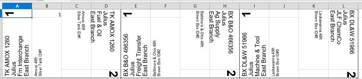
My recommendation is to print blank car-card envelopes and put the car identifications on the car-card waybills. If that recommendation suits you, the referenced spreadsheet is ready for you to use. Sheet 3 will print waybills for 12 cars at a time, starting with the one whose index is placed in cell B1. The illustration below shows design details for the first three waybills, selected by placing a 1 in cell B1. To select the second 12 waybills, set B1 to 12. The value of B1 itself and the faint lines used in the design illustration below will not be printed on the actual waybills. When you are ready, select File – Print. Then cut the printed waybills apart on the solid lines and place them in Sheet 2 envelopes.
Following are the steps to reproduce Sheet 3 using LibreOffice Calc and some suggestions on how to modify it if you want a different waybill design.
The VLOOKUP function
The main reason to use a spreadsheet is that the VLOOKUP function can copy data from the car inventory (Sheet 1) into the waybills (Sheet 3). This means only two general purpose waybill sheets (for two sided waybills) have to be formatted as opposed to having to format a waybill for each car separately. This enables the same waybill sheet to be printed repeatedly, selecting different cars from Sheet 1 for each run.
Set up the basic page format
To make your own spreadsheet file. Use the bottom menu in LibreOffice Calc to create or select Sheet 3. Select Format - Page Style - Page. Set Orientation to Landscape. Set Margins to 0.25. Select Header. and turn the header off. Select Footer and turn the footer off. Click OK.
Set Waybill cell sizes
The illustration above shows the outline of the first waybill in columns A – D, and rows 1 – 3. To format the spreadsheet cells as shown, set the width of columns A – L to 0.86 (a little less than 7/8 inch). This is ¼ the height of a waybill that will fit in a car-card envelope. Each waybill is formed using three rows with heights of 0.25, 1.5, and 0.25. This enables the parts of the waybills to be shown in different font sizes, selected from different columns of Sheet 1, and printed in different directions. When printed, there will be three rows of four-column wide waybills on each side of the paper (front and back).
Merge the cells that will hold car and position data
This is done primarily for appearance and space usage. It is important to merge the cells before entering any data.
Select cells A2 and A3. Select Format – Merge and Unmerge Cells – Merge Cells. This will enable text started in A3 to run over into A2. Repeat this for columns B,E,F,I,and J merging rows 2+3, 5+6, 8+9, 11+12, 14+15, 17+18, 20+21, and 23+24. This is all the cells that will have text rotated to the left.
Repeat again for columns C,D,G,H,K and L merging rows 1+2, 4+5, 7+8, 10+11, 13+14, 16+17, 19+20, and 22+23. This is all the cells that will have text rotated to the right.
One at a time, highlight each group of cells that will represent one waybill (e.g., Cells A1 through D3). For each group select Format – Cells - Borders. Click the second Presets box (outside border only). This highlights the borders around the waybills where they will be cut from the others on the page. Also this enables you to hold the printed page up to the light to be sure the borders are printed in the same place on both sides of the paper.
Insert waybill position numbers
Each waybill has 4 position numbers in bold text to help operators turn the waybills to the next destination when a car is moved. Enter 1 for the first position in the upper left cell of the front of each waybill (columns A, E, and I, rows 1, 4, 7, and 10). Enter position 3 in the upper left cell of the back of each waybill (rows s 13,16,19, and 22). Enter positions 2 and 4 on the corresponding lower right cells of each waybill.
Set font and rotation and spacing of waybill position numbers
Select all the cells with position 1 or 3. Set the font to Arial 24 pt Bold (or other font that you prefer). Select Format – Cells – Alignment. Set Horizontal to Left, Degrees to 90, and Text Direction to Right-to-left (RTL). Select Borders and set all the padding values to 2.0 pt (If Synchronize is set, they will all change when you click away from the first one).
Then select all the cells with position 2 or 4. Set Horizontal alignment to Right, Degrees to 270, and Text Direction to Right-to-left (RTL), and Borders to 2.0.
Setting the borders will keep the text a little bit away from the edges of the waybills. Sometimes home printers do not align the front and back sides perfectly and this gives some margin when cutting out the waybills. .
Merging some cells
The provided spreadsheet uses some merged cells to improve the waybill appearance and maximize the amount of space available for the car identification and destination text. In all of the position 1 and 3 parts of the waybills, the middle and bottom cells in the first two columns are merged (e.g., rows 2 and 3 in columns A and B for waybill 1) and in position 1 and 4 parts of the waybills, the top and middle columns are merged (e.g., rows 1 and 2 in columns C and D for waybill 1). To merge cells, highlight the cells to be merged and select Format – Merge and Unmerge Cells – Merge. This must be done before any text is inserted in the cells
The VLOOKUP and CONCATENATE functions
All the remaining text on the waybills comes from using formulas to copy data from Sheet 1 and combine it in the waybill sheet cells. The basic formula is VLOOKUP(Reference,Sheet1.A:G,column,0). Reference is the address of a data value (in Sheet 3) containing the index of the first car in Sheet 1 whose data is to be processed. I use cell B1 for the reference. In the supplied spreadsheet B1 has the initial value of 1. This means that the VLOOKUP function is to get data from the row of Sheet 1 that contains the value 1 (in other words, to get data for the first car in the inventory list). Since Sheet 3 prints data for 12 cars, it will show waybills for the first 12 cars when B1 contains a 1. To show the next 12 cars, you would set B1 to 12. The second argument in VLOOKUP is Sheet1.A:G, which shows where the inventory list is located. This argument will be the same for all uses of VLOOKUP. The column argument specifies which column on Sheet 1 has the data to be returned. A value of 2 means that the data should come from the Car Mark column on Sheet 1 for the car selected based on the value in B1. The final 0 argument means that an empty column should return a blank.
To keep the Sheet 1 index from being printed, Click on cell B1 then select Format – Cells – Cell Protection and highlight the Hide when Printing option.
The CONCATENATE function just combines arguments into a single string. It is used to combine the Car Mark and Destination columns from Sheet 1 in the top waybill cells. CHAR(10) represents a line break. So for example, the formula =CONCATENATE(VLOOKUP(B1,Sheet1.A:G,2,0),Char(10),VLOOKUP(B1,Sheet1.A:G,4,0)) in the first waybill on sheet 3, when B1 contains a 1, gets the Car Mark of the first car from column 2, adds a line break, and adds Destination 1 from column 4.
Write the formulas
To build the spreadsheet you have to write formulas for each text field and insert them into the cells of the waybills where the text should appear. The easiest way to do this is probably to look at and copy the formulas in the provided spreadsheet. Then modify them if desired.
When the formulas are in place, the referenced text will be shown in the waybill cells, but you will need to rotate it, set the desired font, and adjust the borders as described for the envelopes above.
Rotate the text selected by formulas
When this text produced by the formulas looks right, highlight all of the text in the left two columns of of the waybills, and Select Format – Cells – Alignment and set Horizontal to Left, Degrees to 90, and set Text Direction to Right-to-left (RTL). Select Borders ans set the Padding to 4.0 pt. Then Click OK. Now you should see the description of the first car and the first destination for the car rotated to the left for position 1 on the waybills.
Next highlight all of the text in the right two columns and Select Format – Cells – Alignment and set Vertical to Top, Degrees to 270, and set Text Direction to Right-to-left (RTL). Select Borders and set the Padding to 4.0 pt. Then Click OK. Now you should see the description of the first car and the second destination for the car rotated to the right for position 2 on the waybills.
Select Fonts
You can highlight all the cells to have the same font and set them all at once. I like Arial 12 pt for the car name and destinations and Arial 8 pt for the car descriptions.
Possible Modifications
There are several modifications that you might want. If you are planning to put the car identifications on the envelopes, you will probably want to take them off the waybills. In that case you will want to change the size of the waybills so the car information on the envelope can be seen when the waybill is inserted. You probably will want to change the contents of the Sheet 1 Car Description column to say what car type and loading the waybill is to be used for, rather than listing a description of a particular car. Another possibility is to color-code the waybills for different car types to make it easier to find waybills to be inserted in the appropriate envelopes.